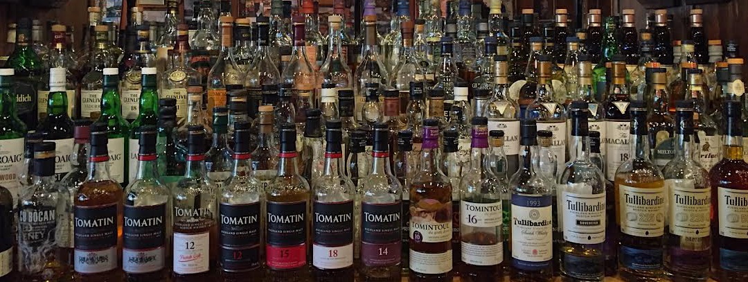
Earlier this month, I went to a bar in Minneapolis called “Merlin’s Rest” with one of the most impressive scotch collections I’ve ever seen compiled into what they called the whisky bible (see: http://merlinsrest.com/whiskywhiskey/the-whisky-bible/). Certain whiskies aged about 30 years ran over $200 for a single pour. This got me thinking a lot about the relationship of the age and price of whisky.

So I did what any reasonable person did and found an API (https://github.com/WhiskeyProject/whiskey-api) to scrape the data and look at the relationship.

Once I gathered the data (for those interested as to how I did that: https://github.com/GWarrenn/whisky/blob/master/whisky.py), the first thing I wanted to do was to run a simple linear regression on price and age to show the relationship between the two.

The output below shows a coefficient of about 5.826, meaning that for every year you add onto a bottle of scotch, the price goes up about $5.83.

y <- whisky_data_w_years$price
x <- whisky_data_w_years$year

initial_model <- lm(y ~ x)

initial_model

## 
## Call:
## lm(formula = y ~ x)
## 
## Coefficients:
## (Intercept)            x  
##     -14.500        5.826

We can then use this model as way to roughly predict what the average 15-year bottle of whisky would cost.

predict(initial_model,data.frame(x=15),interval="confidence")

##        fit      lwr      upr
## 1 72.88727 67.85178 77.92277

And here is the relationship plotted out. The data also contains an average user rating, more on that later.

However, the r-squared for this model isn’t incredibly high, indicating that something other than age is determining the price of the bottle.

summary(initial_model)$r.squared

## [1] 0.363523

Once we control for the region of the whisky’s origin, we see a modest increase in the overall fit of the model. In some regions, like the Scottish Highlands, we see negative coefficients, while regions like Japan and Campbeltown have crazy high coefficients.

y <- whisky_data_w_years$price
x <- whisky_data_w_years$year
r <- whisky_data_w_years$region

model_w_region <- lm(y ~ x + r)

model_w_region

## 
## Call:
## lm(formula = y ~ x + r)
## 
## Coefficients:
##  (Intercept)             x  rCampbeltown     rHighland        rIrish  
##     -19.4036        5.9505       34.3115       -8.0213        1.3721  
##      rIsland        rIslay        rJapan        rOther          rRye  
##      10.7313       -0.8566       28.1602      -22.0025       18.6824  
##    rSpeyside  
##       1.0145

summary(model_w_region)$r.squared

## [1] 0.4378485

We can also use the region to predict the value of an average bottle of 15 year whisky from various parts of the world.

predict(model_w_region,data.frame(x=15,r="Speyside"),interval="confidence")

##        fit      lwr      upr
## 1 70.86852 63.41236 78.32469

predict(model_w_region,data.frame(x=15,r="Japan"),interval="confidence")

##        fit      lwr      upr
## 1 98.01414 74.79607 121.2322

predict(model_w_region,data.frame(x=15,r="Highland"),interval="confidence")

##        fit      lwr      upr
## 1 61.83268 48.09173 75.57363

The next step was to use the rating data that users have contributed along with the prices to segment the whiskies by average price and rating.

Tip: Beware of the top-left and seek out the bottom right.

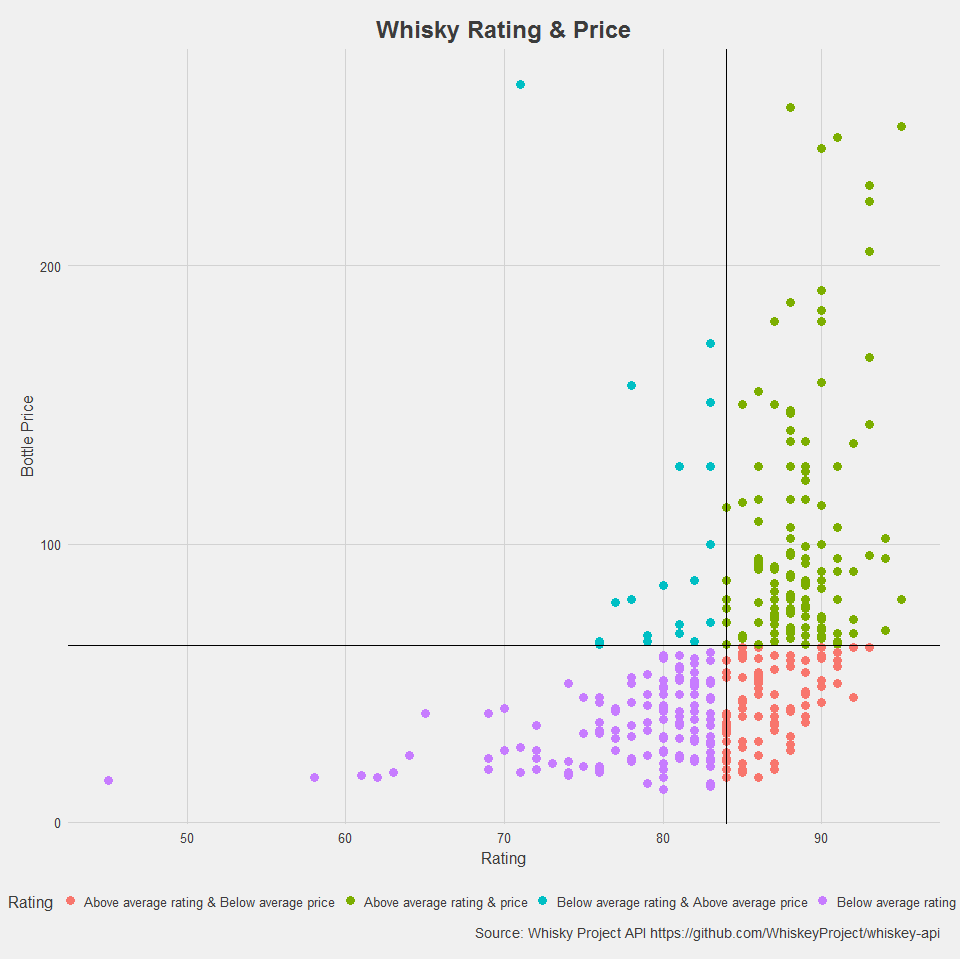
If you’re curious about the outlier data point with one of the higher prices and the very poor rating, it’s the Macallan Rare Cask

Last but not least, I wanted to find good “value” whiskies, or whiskies that are on the lower end of the price spectrum but have generally higher ratings. These whiskies would be ideal candidates for cocktails or if you just need a semi-decent bottle of whisky without breaking the bank (no judgement here). I measured this by dividing the rating by price to create a rough “best value” measure.